This blog won Runner Up Project for the June 2024 BlueDot AI Safety Alignment cohort.
Neural networks with first-order optimisers such as SGD and Adam are the go-to when it comes to training LLMs, forming evaluations, and interpreting models in AI Safety. Meanwhile, optimisation is a hard problem that has been tackled in machine learning in many ways. In this blog, we aim to look at the intersection of interpretability and optimisation, and what it means for the AI safety space. As a brief overview, we’ll consider:
- The problems a model’s optimisation landscape has, and how it affects models and our understanding of them
- How we can interpret said models through activation maximisation
- The use of different optimisers on different problems and interpretability tasks
We’ll look deeply into these things to better understand models and optimisation procedures, and see if we can tie these things together to get a better idea of how things work for AI safety.
The code for this can be found on my at my Github - it involves a general feature visualisation generator that works on a variety of models, datasets, and optimisers and also supports training and checkpointing. Enjoy!
Background and Motivation
Recently, Anthropic came out with its A1 dictionary learning. Dictionary learning, a technique that involves learning a sparse representation of the data, is known to have saddle points.
What is a saddle point?
A saddle point is a point in the function where the gradient at that point is 0, but the point is neither a local minima nor a local maxima. In addition to this, it is where the curvature of some directions are positive, and others are negative.
Saddle points are a commonly re-occuring theme in the loss landscapes of models - in which first order optimisers such as SGD and Adam have trouble navigating through. One of the contributing factors to a standard loss curve plateuing a few iteration in is likely because the model optimisation process is stuck in a saddle point. Here are a two toy examples of saddle functions that I’ve visualised.
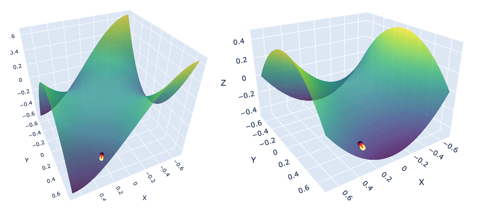 Left: Monkey Saddle defined as $z = x^3 - 3xy^2$. Right: Classic Saddle defined as $z = x^2 − y^2$. Both functions were optimised with Momentum SGD for 200 iterations (LR = 0.001, Momentum = 0.90)
But these are just toy examples, what does an actual landscape look like. Let’s find out - the following is a low dimensional projection of the landscape of a ResNet-110.
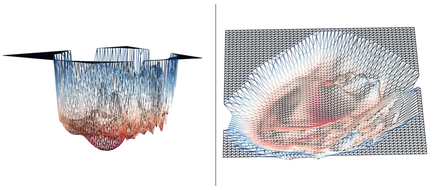 Left: Side view of ResNet-110 projection. Right: Bird’s eye view of ResNet-110 projection. Visualised using neural net loss landscapes.
We can see that while it’s not an exact map to a saddle point, the features that exhibit one still exist, with parts of the landscape being hard to navigate due to plateaus, ragged edges, and pitfalls. So while saddle points exist, even if they’re not exact maps - they’re known to be riddled exponentially throughout the loss landscapes of our models. This is bad because they can:
- Affect the speed at which models train
- Affect the richness of the features that models try to extract
- Plateau the models ability to learn as well as it can by being stuck in a saddle point
Thus, is there a way we can efficiently escape them? This is still an active area of research, but second order optimisers do a pretty good job of this!
How do second order optimisers do this?
Second order optimisers use second order information (the gradient plus more) to map out the curvature of the saddle point. As such, even if the gradient is zero - they can go towards negative curvature directions and escape them by taking larger steps than first order optimisers.
How is this relevant to AI Safety?
You might be wondering how this optimisation research is relevant for AI safety, so let’s tackle that. A big subfield of AI safety is mechanistic interpretability, where we try and understand what models are doing by engineering them to be, (no pun intended), more interpretable! To do this, one of the techniques interpretability researchers use is to look at the features and circuits of models.
Recall in the Zoom In: Circuits paper, we looked at feature visualisation and the universality condition. One way we can tie these together is by extrapolating on their claims with specific regard to optimisers.
Optimisers and Universality
- What effect do different optimisers have on the features?
- Does the universality condition hold for optimisers?
Now, given we also know that saddle points are riddled in the landscape - and these can actively perturb the richness of the features, we ask if this is still the case with second order optimisers.
Feature Visualisations
- Can we utilise second order optimisers to
- a) Engineer model features better?
- b) Extract better features visualisations?
- What does this tell us about the landscape of the feature visualisation task?
The idea is to experiment with first and second order optimisers - and see if features improve or generalise better with specific problem instances. If so, there is potential to use more than just SGD and Adam for training and interpreting models in AI safety. This leads to the key idea of this project.
Experimental Setup and Key Idea
To answer the above questions, we’ll set up three experiments:
Experiments
- Experiment 1: Use first order optimisers on a pre-trained ResNet18 model to visualise features to get a baseline.
- Experiment 2: Train an MNIST MLP and a CIFAR10 3C3L with first and second order optimisers and extract their visualisations
- Experiment 3: Increase the problem difficulty of Experiment 2 with CIFAR100, and see what happens.
To break it down a bit more, the key differences in the experiments are the following:
- In Experiment 1 we’ll use a pre-trained model (ResNet 18 trained on ImageNet 1K), and use activation maximisation to visualise our features with different optimisers (SGD, Adam, AdaGrad)
- In Experiments 2 and 3, we’ll train models with different optimisers (Momentum SGD, Adam, Curveball) and use activation maximisation to visualise features with the same optimiser (AdamW).
This way, we can accurately target the questions we’ve set out to answer. Take a look at how we target them below.
Targets of Experiment 1
Experiment 1 will target Question 3b and 4. It will give us a set of baseline features to work with.
- We can see if the loss landscape of the feature visualisation task can be navigated well.
- If the visualisations need work, this tells us that the landscape for the task could be filled with saddle points and a second order optimiser might extract better visualisations.
Targets of Experiment 2 and 3
Experiments 2 and 3 will target Questions 1, 2, and 3a. By using a mix of first and second order optimisers we can
- Gauge their effects and look at the claim of the universality condition
- See if they engineer features better based on the problem instance
Two final things to note are that:
- The second order optimiser we’re using - which is the Curveball Optimiser (mentioned just above) that’s shown to be quite good at specifically tackling saddle point problems.
- All of the feature visualisations will be done at the last linear layer of these models, since they yield the best visualisations (especially when the model is simple like the MLP or 3C3L).
Experiment 1: Baseline activation maximisation with first order optimisers
In this experiment, we use Momentum SGD, Adam, and AdaGrad to visualise the model features of the following classes from the ImageNet-1K dataset. We’ll use activation maximisation to visualise features for the following classes.
- Spotted Salamander (28)
- Wallaby (104)
- Chihuaua (151)
- Airship (405)
What is activation maximisation?
Activation maximisation is the method of generating the feature visualisations. A lot of people have done projects explaining this and walking through the code - so I won’t go into the nitty gritty, but a brief explanation is that:
- A randomised noisy Gaussian image is passed into a model whose weights are frozen
- An optimiser (like Adam) is used to tweak the image over time to maximise the activations of the model at a particular layer and particular class index of that network
- For better visualisations - different transforms are applied (see code).
- The iterative optimisations result in essentially the features that we get
Visualising these classes gives the following results:
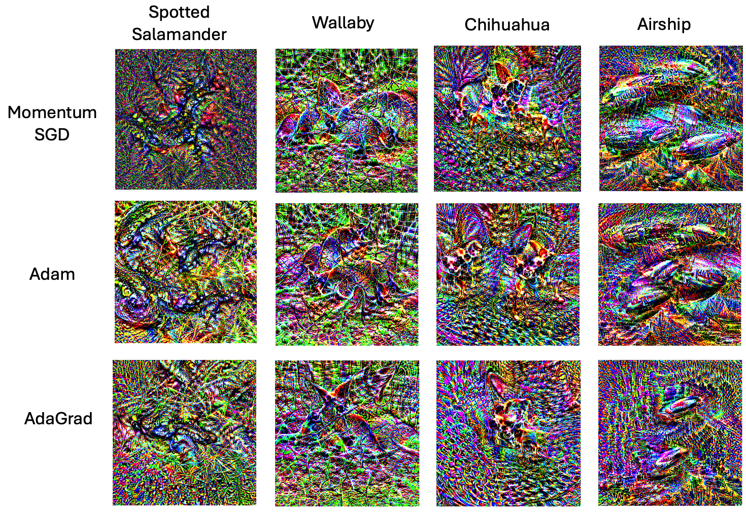 Feature visualisation of different ImageNet classes using Momentum SGD, Adam, and AdaGrad. Each optimiser’s parameters (such as LR, $\alpha$, $\beta$, momentum) were hyper-parameter tuned to ensure that the visualisations produced were fair. The optimisation procedure was run for 1024 iterations.
These visualisations are pretty good! For all the optimisers, we can see that the model interprets these classes well. Visualisations for each class are also similar regardless of the optimiser. This means that all of the optimisers navigate the landscape well enough and reach a point where the activations of the model end up being the same.
But let’s dive a bit deeper, why is this the case? Given we have a pre-trained ResNet-18, it’s quite feature rich as it’s optimised on the ImageNet-1K dataset - so generating features from it will already be good. The architecture of ResNet-18 has a number of “residual” or “skip” connections. These effectively change the landscape to be a lot more navigable, which helps the optimiser maximise the activations even more - resulting in better feature visualisations. See the diagram below, where residual connections make the landscape more convex and less ragged.
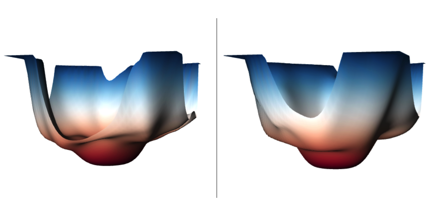 Left: Visualisation of ResNet-18 without residual connections. Right: Visualisation of ResNet-18 with residual connections. Visualised using neural net loss landscapes.
So what can we gain from this?
- The landscape of the feature visualisation task is quite navigable for first order optimisers.
- This is especially the case if we have a feature rich model that is optimised on the task, like this pre-trained ResNet-18 - and the model contains residual connections that make the space more navigable for the optimiser, resulting in more interpretable features.
- Thus, given this problem instance and design, this tells us that first order optimisers do a good job!
Experiment 2: Incorporating second order information
Moving onto Experiment 2, we’ll train an MNIST MLP and a CIFAR10 3C3L model with Momentum SGD, Adam, and Curveball. All optimisers were hyper-parameter tuned (LR, $\alpha$, $\beta$, $\lambda$, momentum) for training.
| MNIST MLP | CIFAR10 3C3L | |
|---|---|---|
| Momentum SGD | 0.9778 | 0.7512 |
| Adam | 0.9831 | 0.7836 |
| Curveball | 0.9812 | 0.8045 |
Then, we’ll generate our visualisations using Adam on the following classes.
| MNIST | CIFAR10 |
|---|---|
| Number 0 | Bird (2) |
| Number 6 | Dog (5) |
| Number 9 | Ship (8) |
The accuracy is an important thing to note here - as it tells us how well the model generalises. We’ll see later when the accuracy drops it becomes harder to visualise features. Visualising the MNIST MLP features gives the following results.
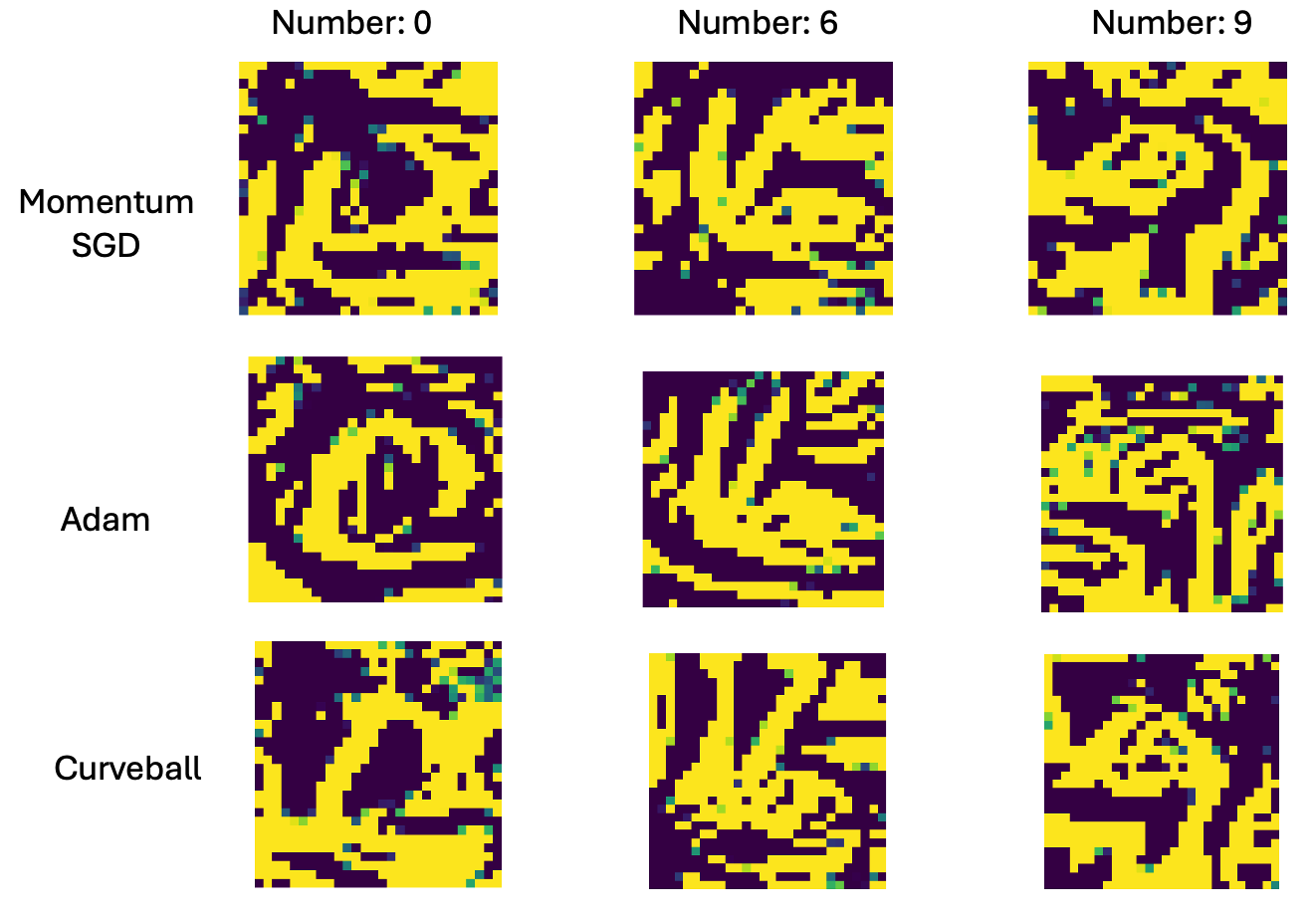 Feature visualisations of MNIST MLP models trained on Momentum SGD, Adam, and Curveball for classes 0, 6 and 9. All optimisers were hyper-parameter tuned with grid search (LR, $\alpha$, $\beta$, $\lambda$, momentum).
MNIST is a simple problem instance - and we can see that as all of the models regardless of the optimiser have accuracy values of 97% or higher. These visualisations are still very interpretable and quite similar. For 0, 6 and 9 - there are clear curve and edge detectors in every case.
Thus, at for a simple MNIST problem - we can conclude that using a second order optimiser doesn’t offer any advantage for engineering features better. It’s likely that the landscape of the MLP is very easy to navigate and generalise - so the features that we extract are just as good regardless of any optimiser.
Given this, let’s up the problem difficulty and use a 3C3L model for CIFAR10 classification. This model doesn’t generalise as well, but this is intentional, as we want to see if we get the same results on a harder problem. We obtain the following results from the 3C3L visualisation.
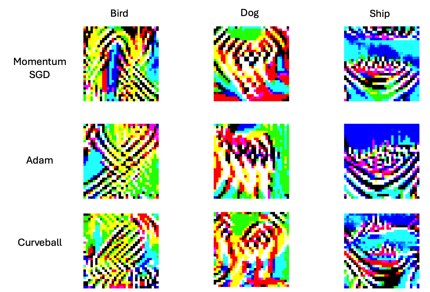
Feature visualisations of CIFAR10 3C3L models trained on Momentum SGD, Adam, and Curveball for bird, dog and ship.
Now we get some more interesting results as the performance drops:
CIFAR10 Feature Visualisation
- Bird: All optimisers seem to extract only the pattern of the wings.
- Dog: Curveball is slightly better than Momentum SGD and Adam, as it recognises the shape of dog’s body, and correctly positions the front and hind legs.
- Ship: Curveball is also better as it recognises the front of the ship compared to Momentum SGD and Adam. It also better connects the front of the ship to the rest of the ship better, unlike Momentum SGD which separates them.
Okay, so we see that given a harder problem instance where the model doesn’t perform as well - the second order optimiser engineers features better in terms of feature visualisations.
Experiment 3: Upping the problem difficulty and extracting features
Let’s see if this is still the case by increasing the problem difficulty. We’ll now train on the CIFAR100 dataset with the same 3C3L model. Again, we tune the hyper-parameters as done in Experiment 2.
| CIFAR100 3C3L | |
|---|---|
| Momentum SGD | 0.3556 |
| Adam | 0.3672 |
| Curveball | 0.3741 |
We visualise on the following classes:
- Dolphin (30)
- Lamp (40)
- Snake (78)
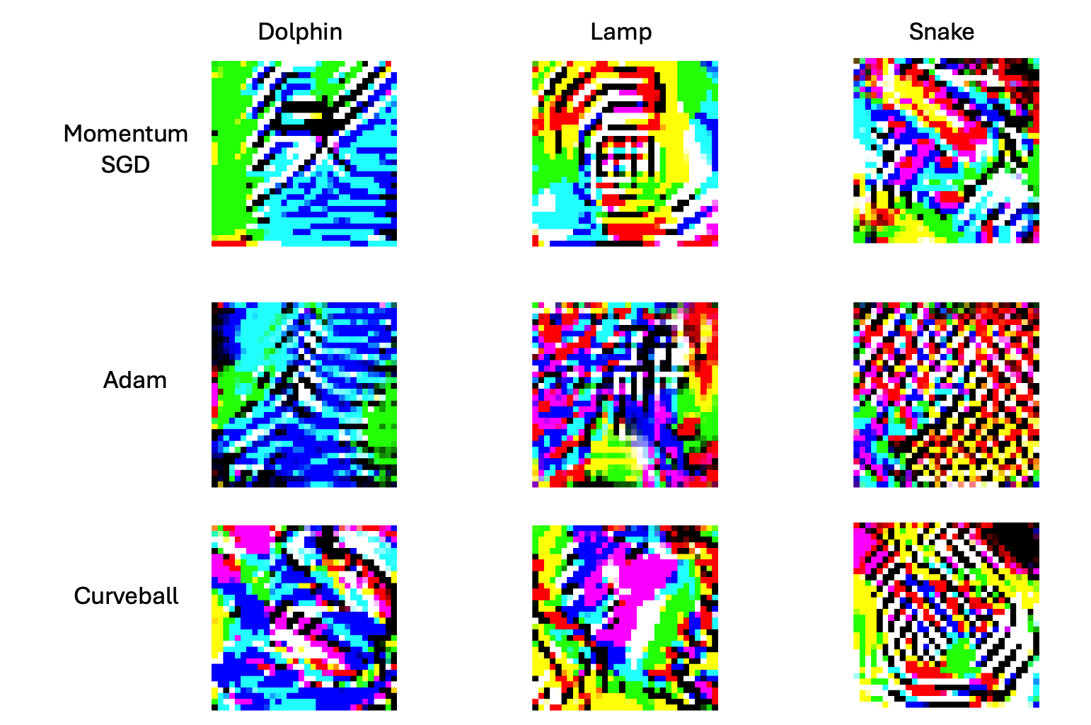 Feature visualisations of CIFAR100 3C3L models trained on Momentum SGD, Adam, and Curveball for dolphin, lamp and snake.
On an even harder problem, we see this even more:
CIFAR100 Feature Visualisation
- Dolphin: Curveball recognises the dolphin body, unlike Momentum SGD and Adam whose interpretations are only the waves.
- Lamp: Curveball shows the lamp body, and the light. Adam is straight noise, and momentum SGD interprets the centre of the lamp.
- Snake: Momentum SGD and Adam are straight noise, while Curveball recognises the body of the snake.
As such, we see that on hard problem instances where the model doesn’t perform well - in which it’s plausible that the model gets stuck in saddle points and hence can’t learn features as well, a second order optimiser can be used to engineer features better.
Discussion
So, what have we found? Let’s address this as answers to the questions we’ve phrased before.
1: What effect do different optimisers have on the features?
We’ve seen that different optimisers can engineer features better depending on the problem instance and the difficulty.
- Given a very navigable space, the feature visualisations were reasonably similar as seen in Experiment 1.
- However, given harder problem instances - we saw that second order optimisers can engineer features better, which we can then visualise.
2: Does the universality condition hold for optimisers?
Yes. We saw in Experiments 2 and 3, even if the second order optimiser had slightly better visualisations - they were still very similar to Adam and SGD for the most part (except for the noisy ones). This shows that the features do tend to be similar even if we’re using different optimisers.
3: Can we utilise second order optimisers to ...
- Engineer model features better?
- Yes! In Experiments 2 and 3, we saw that in harder problem instances where the model doesn’t generalise well (and is possibly stuck in saddle points) - second order optimisers can be used to better engineer features, which we can then visualise.
- In a scenario where we have a black box model and a very hard problem instance, perhaps it’s worth training with a second order optimiser and seeing if the features are better. We can then interpret the features to understand the model better, and then train on SGD or Adam.
- Extract better feature visualisations?
- Also yes! As we can engineer model features better - this results in better feature visualisations, as seen in Experimen 2 and 3.
- Yes! In Experiments 2 and 3, we saw that in harder problem instances where the model doesn’t generalise well (and is possibly stuck in saddle points) - second order optimisers can be used to better engineer features, which we can then visualise.
4: What does this tell us about the landscape of the feature visualisation task?
We saw that in Experiment 1, the feature visualisation task had a very navigable space. The different optimisers resulted in the around the same visualisations. This is thanks to a feature rich model and residual connections which made the space more convex and hence easier to optimise.
Limitations and Future Work
While we find some pretty good results, there are still limitations for this work and directions we can further pursue.
- For all the experiments, it would’ve been great to use another second order optimiser that isn’t saddle point specific like Curveball is, like L-BFGS. I tried getting this to work but unfortunately didn’t L-BFGS is compute intensive.
- Specifically for Experiment 1 - it would’ve been nice to see if the second order optimiser could navigate the same space and produce the same (or better!) feature visualisations. I tried getting Curveball to work but couldn’t.
- Generating feature visualisations for many different classes to further test the hypotheses would be an improvement.
- Visualising the landscape of the MNIST and 3C3L models (as is done for ResNet-110 in the background) would’ve been good to have an insight of what they’re like.
Conclusion
The intersection of optimisation and interpretability is an interesting one, but it’s great to see how these fields influence each other to push the boundaries of AI systems. By improving our understanding of both fields - we can make better interpret models and visualise feature, which will inevitably help in areas of AI safety by making models more aligned and safe.